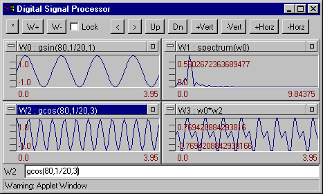
Digital Signal Processor (DSP) is a digital signal processing Java applet designed upon principle integration formulas, signal data set and their graphical presentations. Originally this module was developed as a part of seismic data processing system WSG for Windows 9x/NT/ME/2000/XP and was written in Microsoft Visual C++. Window formulas are the kernel of DSP: any window can contain a formula defining its contents. This formula can reference signal in other Windows, incorporate mathematical functions, and generate signals. In some cases this program is similar to the DADiSP software package. Current version of DSP support up to 16 windows. Also 8 graphics may be overloaded on to the current window.

abs atan ceil conv deriv exp extract floor gcos gline gsin hanning imfft integ kaiser linreg log10 log max mean min refft rand spectrum sqrt tan

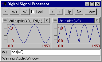
abs(W) - Produces the absolute value of any expression. Example

atan(W) - Calculates the arc-tangent of any expression

ceil(W) - Finds the smallest integer greater than or equal to the input value.

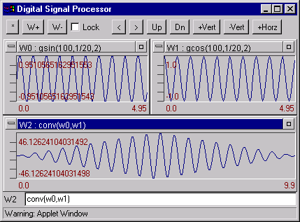
conv(W1, W2) -Convolves two signal W1 and W2. Example

deriv(W) - Derivative of signal W. Calculates by 3 points.

exp(W) - e**W (e=2.71828...)

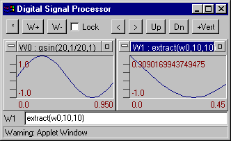
extract(W, start, length) - Makes a new signal by extracting a portion of another signal. Example

floor(W) - Finds the greatest integer less or equal to the input value.

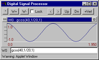
gcos(points, spacing[, n [, j ]]) - Generates a cosine curve cos(2*p *n *t+j ). Example

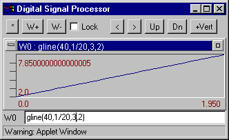
gline(points, spacing, a, b) - Generates a line y=a*t+b. Example

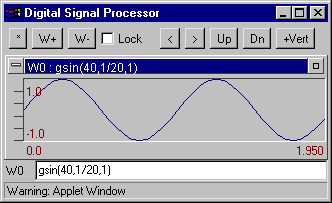
gsin(points, spacing[, n [, j ]]) - Generates a sine curve sin(2*p *n *t+j ). Example

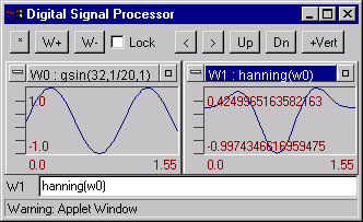
hanning(W) - Multiplies a signal by Hanning Window 0.5*(1.-cos(2*p *i/(nn-1))).

Warning: W padding zeros to signal length will be power of 2. Example

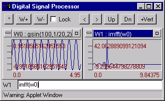
imfft(W) - Imaginary part of the first half of the FFT of the W. W padding zeros to signal length will be power of 2.

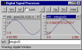
integ(W)- - Calculates the integral of the W. Example

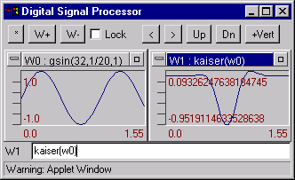
kaiser(W[, b ]) - Multiplies a signal by Kaiser window. W padding zeros to signal length will be power of 2. Example

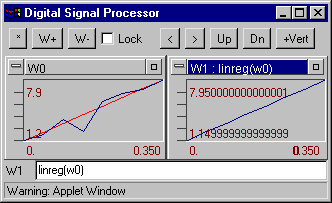
linreg(W) - Determines the best linear fit to a signal. Returns generated line. Example

log10(W) - Calculates the based 10 logarithm of the W.

log(W) - Calculates the natural logarithm of the W.

max(W) - Finds maximum value of the W.

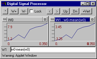
mean(W) - Finds the mean value of the W. Example

min(W) - Finds minimum value of the W.

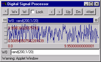
rand(points, spacing) Generates points pseudorandom numbers between 0.0 and 1.0. Example

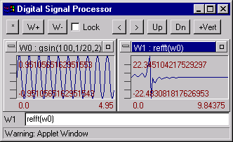
refft(W) - Real part of the first half of the FFT of W. W padding by zeros to signal length will be power of 2.Example

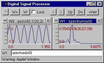
spectrum(W) - Returns the magnitude of the first half of the FFT of a signal. W padding by zeros to signal length will be power of 2. Example

sqrt(W) - Calculates the square root of the W.

tan(W) - Calculates the tangent W.

[*] - Apply formula (Calculate formula in active Window). Equivalent pressing enter key.

[W+] - Add new window.

[W-] - Remove active window.

[Lock] - lock window to protect data associated with active Window from changing. Disable formula editing element.

[>] - Scroll window right.

[<] - Scroll window left.

[Up] - Scroll window up.

[Dn] - Scroll window down.

[+Vert] - Expand vertical.

[-Vert] - Compress vertical.

[+Horz] - Expand horizontal.

[-Horz] - Compress horizontal.

[#] - Fit graphic to window

[Copy] - Copy data from active window to Data Exchange Board.

[Paste] - Paste data from Data Exchange Board to active window.

[Import] - Run dialog box where you can enter your own new data in the ascii format or edit existing data associated with current active window.

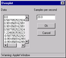
[Overplot] - Overplot a signal from Windows onto current Window.

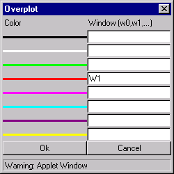
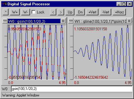
In order to zoom in on a portion of the graphic press Shift button on your keyboard, then press left mouse button on the top corner selected field, then move mouse pointer to the bottom corner and release mouse button. Graphic should be automatically redrawn in new scale.

Example: gsin(40, 1/20, 1) - generates 40 counts of 1Hz sin function with step 1/20=0.05

Example: gcos(40, 1/20, 1) - generates 40 counts of cos function with step 1/20=0.05

Example: gline(40, 1/20, 1, 2) - generates 40 counts of the line 3*t+2 with step 1/20=0.05

Example: extract(w0,10,10) - extract 10 counts from the tenth's point window W0

Example: hanning(w0)

Example: kaiser(w0)

Example: spectrum(w0) spectrum of data from window W0

Example: refft(w0)

Example: imfft(w0)

Example: abs(W0)

Example: integ(w0) - integral of the W0

Example: linreg(w0) - best linear fit to a signal W0

Example: how to remove mean from signal W0

Example: conv(w0, w1) Convolves two signal W0 and W1

Example: rand(200,1/20) - generates 200 pseudorandom numbers.

If you like this applet please download DSP on Java standalone application based on the same technology. To run this software you need JVM 1.2 and above.

Download DSP on Java -> dspjava.jar

After download enter java -jar dspjava.jar to start application.

Andrei Akimov,

Senior Software Engineer, CEME GS RAS

akimov@gsras.ru